Timestamps
RADICAL-Analytics (RA) enables event-based analyses in which the timestamps recorded in a RADICAL-Cybertools (RCT) session are studied as timeseries instead of durations. Those analyses are low-level and, most of the time, useful to ‘visualize’ the process of execution as it happens in one or more components of the stack.
Prologue
Load the Python modules needed to profile and plot a RCT session.
[1]:
import tarfile

import numpy as np
import pandas as pd
import matplotlib as mpl
import matplotlib.pyplot as plt
import matplotlib.ticker as mticker

import radical.utils as ru
import radical.pilot as rp
import radical.analytics as ra

from radical.pilot import states as rps
Load the RADICAL Matplotlib style to obtain viasually consistent and publishable-qality plots.
[2]:
plt.style.use(ra.get_mplstyle('radical_mpl'))
Usually, it is useful to record the stack used for the analysis.
[3]:
! radical-stack
  python               : /home/docs/checkouts/readthedocs.org/user_builds/radicalanalytics/envs/stable/bin/python3
  pythonpath           :
  version              : 3.9.15
  virtualenv           :

  radical.analytics    : 1.34.0-v1.34.0@HEAD-detached-at-0b58be0
  radical.entk         : 1.33.0
  radical.gtod         : 1.20.1
  radical.pilot        : 1.34.0
  radical.saga         : 1.34.0
  radical.utils        : 1.33.0
Event Model
RCT components have each a well-defined event model:
Each event belongs to an entity and is timestamped within a component. The succession of the same event over time constitutes a time series. For example, in RP the event schedule_ok belongs to a task and is timestamped by AgentSchedulingComponent. The timeseries of that event indicates the rate at which tasks are scheduled by RP.
Timestamps analysis
We use RA to derive the timeseries for one or more events of interest. We then plot each time series singularly or together in the same plot. When plotting the time series of multiple events together, they must all be ordered in the same way. Typically, we sort the entities by the timestamp of their first event.
Here is the RA workflow for a timestamps analysis:
- Go at RADICAL-Pilot (RP) event model, RP state model or RADICAL-EnsembleToolkit (EnTK) event model and derive the list of events of interest.
- Convert events and states in RP/RA dict notation.
E.g., a scheduling event and state in RP:
- AGENT_SCHEDULING - picked up by agent scheduler, attempts to assign cores for execution
- AGENT_EXECUTING - picked up by the agent executor and ready to be launched
[4]:
state_sched = {ru.STATE: rps.AGENT_SCHEDULING}
state_exec = {ru.STATE: rps.AGENT_EXECUTING}
- Filter a RCT session for the entity to which the selected event/state belong.
- use
ra.entity.timestamps()and the defined event/state to derive the time series for that event/state.
Session
Name and location of the session we profile.
[5]:
sidsbz2 = !find sessions -maxdepth 1 -type f -exec basename {} \;
sids = [s[:-8] for s in sidsbz2]
sdir = 'sessions/'
Unbzip and untar the session.
[6]:
sidbz2 = sidsbz2[0]
sid = sidbz2[:-8]
sp  = sdir + sidbz2

tar = tarfile.open(sp, mode='r:bz2')
tar.extractall(path=sdir)
tar.close()
Create a ra.Session object for the session. We do not need EnTK-specific traces so load only the RP traces contained in the EnTK session. Thus, we pass the 'radical.pilot' session type to ra.Session.
ra.Session in capt to avoid polluting the notebook with warning messages.[7]:
%%capture capt

sp = sdir + sid

session = ra.Session(sp, 'radical.pilot')
pilots  = session.filter(etype='pilot', inplace=False)
tasks   = session.filter(etype='task' , inplace=False)
We usually want to collect some information about the sessions we are going to analyze. That information is used for bookeeping while performing the analysis (especially when having multiple sessions) and to add meaningful titles to (sub)plots.
[8]:
sinfo = {}

sinfo.update({
    'cores_node': session.get(etype='pilot')[0].cfg['resource_details']['rm_info']['cores_per_node'],
    'pid'       : pilots.list('uid'),
    'ntask'     : len(tasks.get())
})

sinfo.update({
    'ncores'    : session.get(uid=sinfo['pid'])[0].description['cores'],
    'ngpus'     : pilots.get(uid=sinfo['pid'])[0].description['gpus']
})

sinfo.update({
    'nnodes'    : int(sinfo['ncores']/sinfo['cores_node'])
})
Use ra.session.get() on the filtered session objects that contains only task entities. Then use ra.entity.timestamps() to derive the time series for each event/state of interest. We put the time series into a pandas DataFrame to make plotting easier.
[9]:
tseries = {'AGENT_SCHEDULING': [],
           'AGENT_EXECUTING': []}

for task in tasks.get():
    ts_sched = task.timestamps(event=state_sched)[0]
    ts_exec = task.timestamps(event=state_exec)[0]
    tseries['AGENT_SCHEDULING'].append(ts_sched)
    tseries['AGENT_EXECUTING'].append(ts_exec)

time_series = pd.DataFrame.from_dict(tseries)
time_series
[9]:
| AGENT_SCHEDULING | AGENT_EXECUTING | |
|---|---|---|
| 0 | 57.458064 | 1132.290056 |
| 1 | 57.458064 | 696.452034 |
| 2 | 57.458064 | 779.445003 |
| 3 | 57.458064 | 865.469337 |
| 4 | 57.458064 | 732.306301 |
| ... | ... | ... |
| 2043 | 57.722614 | 3084.190474 |
| 2044 | 57.722614 | 377.477711 |
| 2045 | 57.722614 | 732.306301 |
| 2046 | 57.722614 | 1137.071288 |
| 2047 | 57.722614 | 2164.869668 |
2048 rows × 2 columns
Usually, time series are plotted as lineplots but, in our case, we want to plot just the time stamps without a ‘line’ connecting those events, a potentially misleading artefact. Thus, we use a scatterplot in which the X axes are the number of tasks and the Y axes time in seconds. This somehow ‘stretches’ the meaning of a scatterplot as we do not use it to represent a correlation.
zero) we subtract it to the whole time series. Pandas’ dataframe make that easy. We also add 1 to the index we use for the X axes so to start to count tasks from 1 instead of 0.[10]:
fig, ax = plt.subplots(figsize=(ra.get_plotsize(212)))

# Find the min timestamp of the first event/state timeseries and use it to zero
# the Y axes.
zero = time_series['AGENT_SCHEDULING'].min()

ax.scatter(time_series['AGENT_SCHEDULING'].index + 1,
           time_series['AGENT_SCHEDULING'] - zero,
           marker = '.',
           label = ra.to_latex('AGENT_SCHEDULING'))
ax.scatter(time_series['AGENT_EXECUTING'].index + 1,
           time_series['AGENT_EXECUTING'] - zero,
           marker = '.',
           label = ra.to_latex('AGENT_EXECUTING'))

ax.legend(ncol=1, loc='upper left', bbox_to_anchor=(0,1.25))
ax.set_xlabel('Number of Tasks')
ax.set_ylabel('Time (s)')
[10]:
Text(0, 0.5, 'Time (s)')
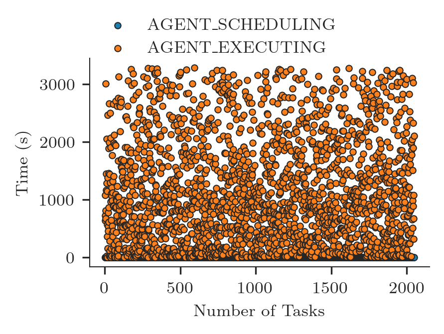
The plot above shows that all the tasks arrive at RP’s Scheduler together (AGENT_SCHEDULING state). That is expected as tasks are transferred in bulk from RP Client’s Task Manager to RP Agent’s Staging In component.
The plot shows that tasks are continously scheduled across the whole duration of the execution (schedule_ok event). That is expected as we have more tasks than available resurces and task wait in the scheduler queue to be scheduled until enough resource are available. Every time one of the task terminates, a certain amount of resources become available. When enough resources become available to execute a new task, the scheduler schedule the task that, then executes on those resources.
The plot above might be confusing because tasks are not ordered by the time in which they were scheduled. We sort time_series by AGENT_EXECUTING and then we plot the scatterplot again,
[11]:
ts_sorted = time_series.sort_values(by=['AGENT_EXECUTING']).reset_index(drop=True)
ts_sorted
[11]:
| AGENT_SCHEDULING | AGENT_EXECUTING | |
|---|---|---|
| 0 | 57.458064 | 57.669098 |
| 1 | 57.458064 | 57.676626 |
| 2 | 57.458064 | 57.684323 |
| 3 | 57.458064 | 57.691968 |
| 4 | 57.458064 | 57.717011 |
| ... | ... | ... |
| 2043 | 57.458064 | 3325.463749 |
| 2044 | 57.458064 | 3325.463749 |
| 2045 | 57.458064 | 3333.839660 |
| 2046 | 57.722614 | 3333.839660 |
| 2047 | 57.458064 | 3338.267327 |
2048 rows × 2 columns
[12]:
fig, ax = plt.subplots(figsize=(ra.get_plotsize(212)))

# Find the min timestamp of the first event/state timeseries and use it to zero
# the Y axes.
zero = ts_sorted['AGENT_SCHEDULING'].min()

ax.scatter(ts_sorted['AGENT_SCHEDULING'].index + 1,
           ts_sorted['AGENT_SCHEDULING'] - zero,
           marker = '.',
           label = ra.to_latex('AGENT_SCHEDULING'))
ax.scatter(ts_sorted['AGENT_EXECUTING'].index + 1,
           ts_sorted['AGENT_EXECUTING'] - zero,
           marker = '.',
           label = ra.to_latex('AGENT_EXECUTING'))

ax.legend(ncol=1, loc='upper left', bbox_to_anchor=(0,1.25))
ax.set_xlabel('Number of Tasks')
ax.set_ylabel('Time (s)')
[12]:
Text(0, 0.5, 'Time (s)')
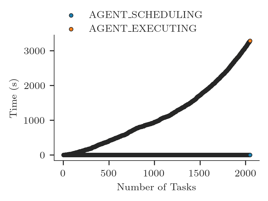
Unsurprisingly, the resulting plot is consistent with the plot shown in Concurrency.
Adding execution events to our timestamps analysis should confirm the duration distributions of the time taken by RP’s Executor launch method to launch tasks. We add the relevant events/states to the time_series dataframe and we sort it again for the AGENT_EXECUTING event.
[13]:
executor = {
    'rank_start'     : {ru.EVENT: 'rank_start'},
    'rank_stop'      : {ru.EVENT: 'rank_stop'}
}

for name, event in executor.items():

    tseries = []
    for task in tasks.get():
        ts_state = task.timestamps(event=event)[0]
        tseries.append(ts_state)

    time_series[name] = tseries

ts_sorted = time_series.sort_values(by=['AGENT_EXECUTING']).reset_index(drop=True)
ts_sorted
[13]:
| AGENT_SCHEDULING | AGENT_EXECUTING | rank_start | rank_stop | |
|---|---|---|---|---|
| 0 | 57.458064 | 57.669098 | 57.848533 | 68.974868 |
| 1 | 57.458064 | 57.676626 | 57.884947 | 64.122034 |
| 2 | 57.458064 | 57.684323 | 57.883325 | 63.967687 |
| 3 | 57.458064 | 57.691968 | 57.989414 | 63.107628 |
| 4 | 57.458064 | 57.717011 | 58.008192 | 66.338753 |
| ... | ... | ... | ... | ... |
| 2043 | 57.458064 | 3325.463749 | 3325.541283 | 3333.749098 |
| 2044 | 57.458064 | 3325.463749 | 3325.562549 | 3327.760062 |
| 2045 | 57.458064 | 3333.839660 | 3333.918936 | 3335.097386 |
| 2046 | 57.722614 | 3333.839660 | 3333.904375 | 3338.089182 |
| 2047 | 57.458064 | 3338.267327 | 3338.346752 | 3343.485991 |
2048 rows × 4 columns
We plot the new time series alongside the previous ones.
[14]:
fig, ax = plt.subplots(figsize=(ra.get_plotsize(212)))

zero = ts_sorted['AGENT_SCHEDULING'].min()

for ts in ts_sorted.columns:
    ax.scatter(ts_sorted[ts].index + 1,
               ts_sorted[ts] - zero,
               marker = '.',
               label = ra.to_latex(ts))

ax.legend(ncol=2, loc='upper left', bbox_to_anchor=(-0.25,1.5))
ax.set_xlabel('Number of Tasks')
ax.set_ylabel('Time (s)')
[14]:
Text(0, 0.5, 'Time (s)')
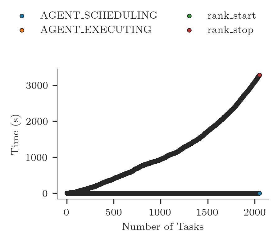
At the resolution of this plot, all the states and events AGENT_SCHEDULING, AGENT_EXECUTING, rank_start and rank_stop overlap. That indicates that the duration of each task is very short and, thus, the scheduling turnover is very rapid.
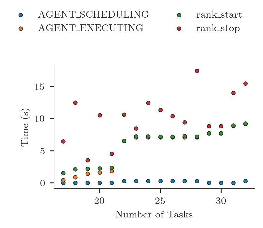
In presence of a large amount of tasks, we can slice the time stamps to plot one or more of their subsets.
[15]:
fig, ax = plt.subplots(figsize=(ra.get_plotsize(212)))

# Slice time series to plot only one of their subsets
ts_sorted = ts_sorted.reset_index(drop=True)
ts_sorted = ts_sorted.iloc[16:32]

zero = ts_sorted['AGENT_SCHEDULING'].min()

for ts in ts_sorted.columns:
    ax.scatter(ts_sorted[ts].index + 1,
               ts_sorted[ts] - zero,
               marker = '.',
               label = ra.to_latex(ts))

ax.legend(ncol=2, loc='upper left', bbox_to_anchor=(-0.25,1.5))
ax.set_xlabel('Number of Tasks')
ax.set_ylabel('Time (s)')
[15]:
Text(0, 0.5, 'Time (s)')