Duration

In RADICAL-Analytics (RA), duration is a general term to indicate a measure of the time spent by an entity (local analyses) or a set of entities (global analyses) between two timestamps. For example, data staging, scheduling, pre-executing, and executing time of one or more tasks; description, submission and execution time of one or more pipelines or stages; and runtime of one or more pilots.

We show two sets of default durations for RADICAL-Pilot (RP) and how to define arbitrary durations, depending on the specifics of a given analysis. We then see how to plot the most common durations

Prologue

Load the Python modules needed to profile and plot a RADICAL-Cybertool (RCT) session.

import os
import tarfile

import numpy as np
import pandas as pd
import matplotlib as mpl
import matplotlib.pyplot as plt
import matplotlib.ticker as mticker

import radical.utils as ru
import radical.pilot as rp
import radical.analytics as ra

from radical.pilot import states as rps

Load the RADICAL Matplotlib style to obtain viasually consistent and publishable-qality plots.

plt.style.use(ra.get_mplstyle('radical_mpl'))

Usually, it is useful to record the stack used for the analysis.

Note: The analysis stack might be different from the stack used to create the session to analyze. Usually, the two stacks must have the same minor release number (Major.Minor.Patch) in order to be compatible.

! radical-stack

  python               : /home/docs/checkouts/readthedocs.org/user_builds/radicalanalytics/envs/stable/bin/python3
  pythonpath           :
  version              : 3.9.15
  virtualenv           :

  radical.analytics    : 1.34.0-v1.34.0@HEAD-detached-at-0b58be0
  radical.entk         : 1.33.0
  radical.gtod         : 1.20.1
  radical.pilot        : 1.34.0
  radical.saga         : 1.34.0
  radical.utils        : 1.33.0

Default Durations

Currently, we offer a set of default durations for pilot and task entities of RP.

pd.DataFrame(ra.utils.tabulate_durations(rp.utils.PILOT_DURATIONS_DEBUG))

	Duration Name	Start Timestamp	Stop Timestamp
0	p_pmgr_create	NEW	PMGR_LAUNCHING_PENDING
1	p_pmgr_launching_init	PMGR_LAUNCHING_PENDING	PMGR_LAUNCHING
2	p_pmgr_launching	PMGR_LAUNCHING	staging_in_start
3	p_pmgr_stage_in	staging_in_start	staging_in_stop
4	p_pmgr_submission_init	staging_in_stop	submission_start
5	p_pmgr_submission	submission_start	submission_stop
6	p_pmgr_scheduling_init	submission_stop	PMGR_ACTIVE_PENDING
7	p_pmgr_scheduling	PMGR_ACTIVE_PENDING	bootstrap_0_start
8	p_agent_ve_setup_init	bootstrap_0_start	ve_setup_start
9	p_agent_ve_setup	ve_setup_start	ve_setup_stop
10	p_agent_ve_activate_init	ve_setup_stop	ve_activate_start
11	p_agent_ve_activate	ve_activate_start	ve_activate_stop
12	p_agent_install_init	ve_activate_stop	rp_install_start
13	p_agent_install	rp_install_start	rp_install_stop
14	p_agent_launching	rp_install_stop	PMGR_ACTIVE
15	p_agent_terminate_init	PMGR_ACTIVE	cmd
16	p_agent_terminate	cmd	bootstrap_0_stop
17	p_agent_finalize	bootstrap_0_stop	DONE, CANCELED, FAILED
18	p_agent_runtime	bootstrap_0_start	bootstrap_0_stop

pd.DataFrame(ra.utils.tabulate_durations(rp.utils.TASK_DURATIONS_DEBUG))

	Duration Name	Start Timestamp	Stop Timestamp
0	t_tmgr_create	NEW	TMGR_SCHEDULING_PENDING
1	t_tmgr_schedule_queue	TMGR_SCHEDULING_PENDING	TMGR_SCHEDULING
2	t_tmgr_schedule	TMGR_SCHEDULING	TMGR_STAGING_INPUT_PENDING
3	t_tmgr_stage_in_queue	TMGR_STAGING_INPUT_PENDING	TMGR_STAGING_INPUT
4	t_tmgr_stage_in	TMGR_STAGING_INPUT	AGENT_STAGING_INPUT_PENDING
5	t_agent_stage_in_queue	AGENT_STAGING_INPUT_PENDING	AGENT_STAGING_INPUT
6	t_agent_stage_in	AGENT_STAGING_INPUT	AGENT_SCHEDULING_PENDING
7	t_agent_schedule_queue	AGENT_SCHEDULING_PENDING	AGENT_SCHEDULING
8	t_agent_schedule	AGENT_SCHEDULING	AGENT_EXECUTING_PENDING
9	t_agent_execute_queue	AGENT_EXECUTING_PENDING	AGENT_EXECUTING
10	t_agent_execute_prepare	AGENT_EXECUTING	task_mkdir
11	t_agent_execute_mkdir	task_mkdir	task_mkdir_done
12	t_agent_execute_layer_start	task_mkdir_done	task_run_start
13	t_agent_execute_layer	task_run_start	task_run_ok
14	t_agent_lm_start	task_run_start	launch_start
15	t_agent_lm_submit	launch_start	exec_start
16	t_agent_lm_execute	exec_start	exec_stop
17	t_agent_lm_stop	exec_stop	task_run_stop
18	t_agent_stage_out_start	task_run_stop	AGENT_STAGING_OUTPUT_PENDING
19	t_agent_stage_out_queue	AGENT_STAGING_OUTPUT_PENDING	AGENT_STAGING_OUTPUT
20	t_agent_stage_out	AGENT_STAGING_OUTPUT	TMGR_STAGING_OUTPUT_PENDING
21	t_agent_push_to_tmgr	TMGR_STAGING_OUTPUT_PENDING	TMGR_STAGING_OUTPUT
22	t_tmgr_destroy	TMGR_STAGING_OUTPUT	DONE, CANCELED, FAILED
23	t_agent_unschedule	unschedule_start	unschedule_stop

Most of those default durations are meant for debugging. They are as granular as possible and (almost completely) contiguous. Only few of them are commonly used in experiment analyses. For example:

• p_agent_runtime: the amount of time for which one or more pilots (i.e., RP Agent) were active.
• p_pmngr_scheduling: the amount of time one or more pilots waited in the queue of the HPC batch system.
• t_agent_stage_in: the amount of time taken to stage the input data of one or more tasks.
• t_agent_schedule: the amount of time taken to schedule of one or more tasks.
• t_agent_t_pre_execute: the amount of time taken to execute the pre_exec of one or more tasks.
• t_agent_t_execute: the amount of time taken to execute the executable of one or more tasks.
• t_agent_t_stage_out: the amount of time taken to stage the output data of one or more tasks.

Arbitrary Durations

RA enables the arbitrary definition of durations, depending on the analysis requirements. For example, given an experiment to characterize the performance of one of RP’s executors, it might be useful to measure the amount of time spent by each task in RP’s Executor component.

Warning: Correctly defining a duration requires a detailed understanding of both RP architecture and event model.

Once we acquired an understanding of RP architecture and event model, we can define our duration as the sum of the time spent by tasks in RP’s Executor component, before and after the execution of the tasks’ executable.

t_executor_before = [{ru.STATE: rps.AGENT_EXECUTING},
                     {ru.EVENT: 'rank_start'} ]

t_executor_after  = [{ru.EVENT: 'rank_stop'},
                     {ru.EVENT: 'task_run_stop'} ]

Duration Analysis

Every analysis with RA requires to load the traces produced by RP or RADICAL-EnsembleToolkit (EnTK) into a session object. Both RP and EnTK write traces (i.e., timestamped and annotated sequences of events) to a directory called client sandbox. This directory is created inside the directory from which the application executed. The name of the client sandbox is a session ID, e.g., rp.session.hostname.username.000000.0000 for RP and en.session.hostname.username.000000.0000 for EnTK.

Session

Name and location of the session we profile.

sidsbz2 = !find sessions -maxdepth 1 -type f -exec basename {} \;
sids = [s[:-8] for s in sidsbz2]
sdir = 'sessions/'

Unbzip and untar the session.

sidbz2 = sidsbz2[0]
sid = sidbz2[:-8]
sp  = sdir + sidbz2

tar = tarfile.open(sp, mode='r:bz2')
tar.extractall(path=sdir)
tar.close()

Create a ra.Session object for the session. We do not need EnTK-specific traces so load only the RP traces contained in the EnTK session. Thus, we pass the 'radical.pilot' session type to ra.Session.

Warning: We already know we need information about pilots and tasks. Thus, we save in memory two session objects filtered for pilots and tasks. This might be too expensive with large sessions, depending on the amount of memory available.

Note: We save the ouput of ra.Session in capt to avoid polluting the notebook with warning messages.

%%capture capt

sp = sdir + sid
display(sp)

session = ra.Session(sp, 'radical.pilot')
pilots  = session.filter(etype='pilot', inplace=False)
tasks   = session.filter(etype='task' , inplace=False)

As seen above, each duration measures the time spent by an entity (local analyses) or a set of entities (global analyses) between two timestamps.

We starts with a global analysis to measure for how long all the pilots of a session have been active. Looking at RP’s event model of the pilot entity and to rp.utils.PILOT_DURATIONS_DEBUG, we know that a pilot is active between the events bootstrap_0_start and bootstrap_0_stop. We also know that we have a default duration with those events: p_agent_runtime.

To measure that duration, first, we filter the session object so to keep only the entities of type Pilot; and, second, we get the cumulative amount of time for which all the pilot were active. It is that cumulative measure that defines this analysis as global.

p_runtime = pilots.duration(event=rp.utils.PILOT_DURATIONS_DEBUG['p_agent_runtime'])
p_runtime

3327.484554052353

Note: ra.session.duration works with a set of pilots, including the case in which we have a single pilot. If we have a single pilot, the cumulative active time of all the pilots is equal to the active time of the only available pilot.

If we have more than one pilot and we want to measure the active time of only one of them, then we need to perform a local analysis. A rapid way to get a list of all the pilot entities in the session and, for example, see their unique identifiers (uid) is:

puids = [p.uid for p in pilots.get()]
puids

['pilot.0000']

Once we know the ID of the pilot we want to analyze, first we filter the session object so to keep only the pilot we want to analyze; and, second, we get the amount of time for which that specific pilot was active:

p0000 = pilots.filter(uid='pilot.0000')
p0000_runtime = p0000.duration(event=rp.utils.PILOT_DURATIONS_DEBUG['p_agent_runtime'])
p0000_runtime

3327.484554052353

The same approach and both global and local analyses can be used for every type of entity supported by RA (currently: pilot, task, pipeline, and stage).

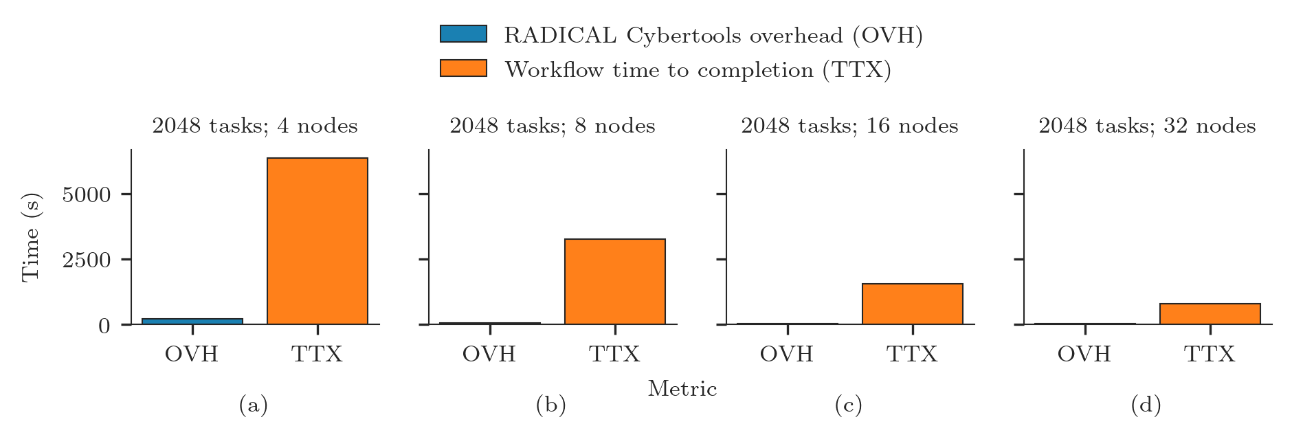
Total task execution time (TTX) and RCT overheads (OVH) are among the most common metrics used to describe the global behavior of RCT. TTX measures the time taken by ALL the tasks to execute, accounting for their cocurrency. This means that if Task_a and task_b both start at the same time and Task_a terminates after 10 minutes and Task_b after 15, TTX will be 15 minutes. Conversely, if task_b starts to execute 5 minutes after task_a, TTX will be 20 minutes. Finally, if task_b starts to execute 10 minutes after task_a terminated, TTX will be 25 minutes as the gap between the two tasks will not be considered.

ttx = tasks.duration(event=rp.utils.TASK_DURATIONS_DEBUG['t_agent_lm_execute'])
ovh = p_runtime - ttx

print('TTX: %f\nOVH: %f' % (ttx, ovh))

TTX: 3267.044225
OVH: 60.440329

Plotting

We plot TTX and OVH for 4 sessions of an experiment. We create suitable data structures to suppor the plotting and we produce a figure with 4 subplots. Unbzip and untar those sessions.

for sid in sidsbz2:
    sp = sdir + sid
    tar = tarfile.open(sp, mode='r:bz2')
    tar.extractall(path=sdir)
    tar.close()

Create the session, tasks and pilots objects for each session.

%%capture capt

ss = {}
for sid in sids:
    sp = sdir + sid
    ss[sid] = {'s': ra.Session(sp, 'radical.pilot')}
    ss[sid].update({'p': ss[sid]['s'].filter(etype='pilot'   , inplace=False),
                    't': ss[sid]['s'].filter(etype='task'    , inplace=False)})

Derive the information about each session we need to use in our plots.

for sid in sids:
    ss[sid].update({'cores_node': ss[sid]['s'].get(etype='pilot')[0].cfg['resource_details']['rm_info']['cores_per_node'],
                    'pid'       : ss[sid]['p'].list('uid'),
                    'ntask'     : len(ss[sid]['t'].get())
    })

    ss[sid].update({'ncores'    : ss[sid]['p'].get(uid=ss[sid]['pid'])[0].description['cores'],
                    'ngpus'     : ss[sid]['p'].get(uid=ss[sid]['pid'])[0].description['gpus']
    })

    ss[sid].update({'nnodes'    : int(ss[sid]['ncores']/ss[sid]['cores_node'])})

Use the default global durations to calculate TTX and OVH for each session of the experiment.

for sid in sids:
    t  = ss[sid]['t']
    p  = ss[sid]['p']

    ss[sid].update({
      'ttx': t.duration(event=rp.utils.TASK_DURATIONS_DEBUG['t_agent_lm_execute']),
      'p_runtime': p.duration(event=rp.utils.PILOT_DURATIONS_DEBUG['p_agent_runtime'])
    })

    ss[sid].update({'ovh': ss[sid]['p_runtime'] - ss[sid]['ttx']})

When plotting TTX and OVH in a plot with a subplot for each session, we want the subplots to be ordered by number of nodes. In that way, we will be able to ‘see’ the strong scaling behavior. Thus, we sort sids for number of cores.

sorted_sids = [s[0] for s in sorted(ss.items(), key=lambda item: item[1]['ncores'])]

Plot TTX and OVH for each session, add information about each run and letters for each subplot fo easy referencing in a paper.

nsids = len(sids)

fwidth, fhight = ra.get_plotsize(516,subplots=(1, nsids))
fig, axarr = plt.subplots(1, nsids, sharey=True, figsize=(fwidth, fhight))

i = 0
j = 'a'
for sid in sorted_sids:

    if len(sids) > 1:
        ax = axarr[i]
    else:
        ax = axarr

    ax.title.set_text('%s tasks; %s nodes' % (ss[sid]['ntask'], int(ss[sid]['nnodes'])))

    ax.bar(x = 'OVH', height = ss[sid]['ovh'])
    ax.bar(x = 'TTX', height = ss[sid]['ttx'])

    ax.set_xlabel('(%s)' % j, labelpad=10)

    i = i + 1
    j = chr(ord(j) + 1)

fig.text(  0.05,  0.5 , 'Time (s)', va='center', rotation='vertical')
fig.text(  0.5 , -0.2, 'Metric'  , ha='center')
fig.legend(['RADICAL Cybertools overhead (OVH)',
            'Workflow time to completion (TTX)'],
           loc='upper center',
           bbox_to_anchor=(0.5, 1.5),
           ncol=1)

<matplotlib.legend.Legend at 0x7ffa31934df0>

Danger of Duration Analysis

Warning: Most of the time, the durations of global analyses are NOT additive.

For example, the sum of the total time taken by RP Agent to manage all the tasks and the total amount of time taken to execute all those tasks is greater than the time taken to execute the workload. This is because RP is a distributed system that performs multiple operations at the same time on multiple resources. Thus, while RP Agent manages a task, it might be executing another task.

Consider three durations:

1. t_agent_t_load: the time from when RP Agent receives a compute task to the time in which the compute task’s executable is launched.
2. t_agent_t_execute: default duration for the time taken by a compute task’s executable to execute.
3. t_agent_t_load: the time from when a compute task’s executable finishes to execute to when RP Agent mark the compute task with a final state (DONE, CANCELED or FAILED).

For a single task, t_agent_t_load, t_agent_t_execute and t_agent_t_load are contiguos and therefore additive. A single task cannot be loaded by RP Agent while it is also executed. For multiple tasks, this does not apply: one task might be loaded by RP Agent while another task is being executed.

Distribution of Durations

We want to calculate the statistical distribution of default and arbitrary durations. Variance and outliers characterize the runtime behavior of both tasks and RCT.

Global durations like TTX and OVH are aggregated across all entities: TTX aggregates the duration of each task while OVH that of all the RCT components active when no tasks are executed. For a distribution, we need instead the individual measure for each entity and component. For example, to calculate the distribution of task execution time, we have to measure the execution time of each task.

We use RA to cycle through all the task entities and then the get and duration methods to return the wanted duration for each task. We use both the default duration for task runtime and the two arbitary durations we defined above for the time taken by RP executor to manage the execution of the task.

t_duration = {}
events = {'tx': rp.utils.TASK_DURATIONS_DEBUG['t_agent_lm_execute'],
          't_executor_before': t_executor_before,
          't_executor_after': t_executor_after}

for sid in sorted_sids:
    t_duration[sid] = {}
    for name, event in events.items():
        t_duration[sid].update({name: []})
        for tid in ss[sid]['t'].list('uid'):
            task = ss[sid]['t'].get(etype='task', uid=tid)[0]
            duration = task.duration(event=event)
            t_duration[sid][name].append(duration)

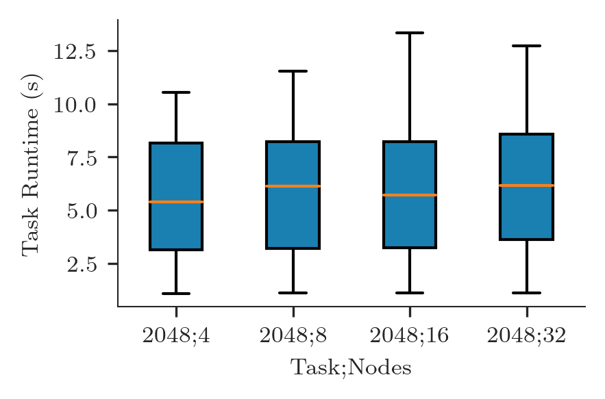
We can now plot the distribution of task execution time as a boxplot for each session:

fwidth, fhight = ra.get_plotsize(212)
fig, ax = plt.subplots(figsize=(fwidth, fhight))

data   = [t_duration[sid]['tx'] for sid in sorted_sids]
labels = ['%s;%s' % (ss[sid]['ntask'], int(ss[sid]['nnodes'])) for sid in sorted_sids]

ax.boxplot(data, labels=labels, patch_artist=True)

ax.set_xlabel('Task;Nodes')
ax.set_ylabel('Task Runtime (s)')

Text(0, 0.5, 'Task Runtime (s)')

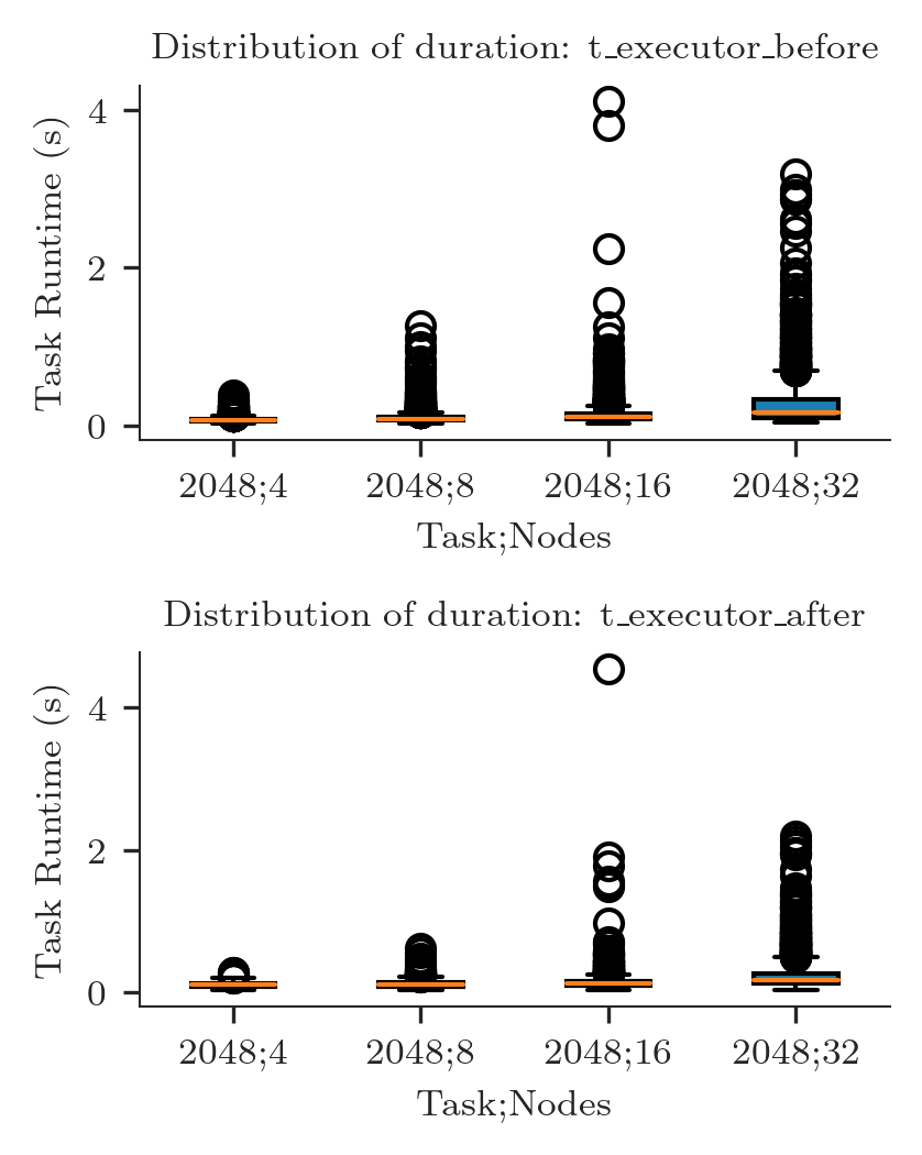
We can do the same for the arbitrary durations defined above: t_executor_before and t_executor_after

fwidth, fhight = ra.get_plotsize(212, subplots=(2, 1))
fig, axarr = plt.subplots(2, 1, figsize=(fwidth, fhight))
plt.subplots_adjust(hspace=0.6)

i = 0
for dname in ['t_executor_before', 't_executor_after']:
    ax = axarr[i]

    data   = [t_duration[sid][dname] for sid in sorted_sids]
    labels = ['%s;%s' % (ss[sid]['ntask'], int(ss[sid]['nnodes'])) for sid in sorted_sids]

    ax.boxplot(data, labels=labels, patch_artist=True)

    ax.set_title('Distribution of duration: %s' % ra.to_latex(dname))
    ax.set_xlabel('Task;Nodes')
    ax.set_ylabel('Task Runtime (s)')

    i += 1