Concurrency

RADICAL-Analytics (RA) offers a method ra.session.concurrency that returns a time series, counting the number of tasks which are matching a given pair of timestamps at any point in time. For example, a time series can show the number of concurrent tasks that were scheduled, executed or staging in/out at every point of time, during the execution of the workload.

We plot concurrency time series as a canonical line plot. We can add to the same plot multiple timeseries, showing the relation among diverse components of each RADICAL-Cybertool (RCT) system.

Prologue

Load the Python modules needed to profile and plot a RCT session.

import os
import tarfile

import pandas as pd
import matplotlib as mpl
import matplotlib.pyplot as plt
import matplotlib.ticker as mticker

import radical.utils as ru
import radical.pilot as rp
import radical.entk as re
import radical.analytics as ra

Load the RADICAL Matplotlib style to obtain viasually consistent and publishable-qality plots.

plt.style.use(ra.get_mplstyle('radical_mpl'))

Usually, it is useful to record the stack used for the analysis.

Note: The analysis stack might be different from the stack used to create the session to analyze. Usually, the two stacks must have the same minor release number (Major.Minor.Patch) in order to be compatible.

! radical-stack

  python               : /home/docs/checkouts/readthedocs.org/user_builds/radicalanalytics/envs/latest/bin/python3
  pythonpath           :
  version              : 3.9.17
  virtualenv           :

  radical.analytics    : 1.35.0-v1.34.0-4-g213a18f@HEAD-detached-at-origin-devel
  radical.entk         : 1.36.0
  radical.gtod         : 1.20.1
  radical.pilot        : 1.36.0
  radical.saga         : 1.36.0
  radical.utils        : 1.33.0

Session

Name and location of the session we profile.

sidsbz2 = !find sessions -maxdepth 1 -type f -exec basename {} \;
sids = [s[:-8] for s in sidsbz2]
sdir = 'sessions/'

Unbzip and untar the session.

sidbz2 = sidsbz2[0]
sid = sidbz2[:-8]
sp  = sdir + sidbz2

tar = tarfile.open(sp, mode='r:bz2')
tar.extractall(path=sdir)
tar.close()

Create a ra.Session object for the session. We do not need EnTK-specific traces so load only the RP traces contained in the EnTK session. Thus, we pass the 'radical.pilot' session type to ra.Session.

Warning: We already know we need information about pilots and tasks. Thus, we save in memory two session objects filtered for pilots and tasks. This might be too expensive with large sessions, depending on the amount of memory available.

Note: We save the ouput of ra.Session in capt to avoid polluting the notebook with warning messages.

%%capture capt

sp = sdir + sid

session = ra.Session(sp, 'radical.pilot')
pilots  = session.filter(etype='pilot', inplace=False)
tasks   = session.filter(etype='task' , inplace=False)

Plotting

We name some pairs of events we want to use for concurrency analysis. We use the ra.session’s concurrency method to compute the number of tasks which match the given pair of timestamps at every point in time. We zero the time of the X axes.

pairs = {'Task Scheduling'  : [{ru.STATE: 'AGENT_SCHEDULING'},
                               {ru.EVENT: 'schedule_ok'     } ],
         'Task Execution'   : [{ru.EVENT: 'rank_start'      },
                               {ru.EVENT: 'rank_stop'       } ]}

time_series = {pair: session.concurrency(event=pairs[pair]) for pair in pairs}

fig, ax = plt.subplots(figsize=(ra.get_plotsize(212)))

for name in time_series:

    zero = min([e[0] for e in time_series[name]])
    x = [e[0]-zero for e in time_series[name]]

    y = [e[1] for e in time_series[name]]
    ax.plot(x, y, label=ra.to_latex(name))

ax.legend(ncol=2, loc='upper left', bbox_to_anchor=(-0.15,1.2))
ax.set_ylabel('Number of Tasks')
ax.set_xlabel('Time (s)')

Text(0.5, 0, 'Time (s)')

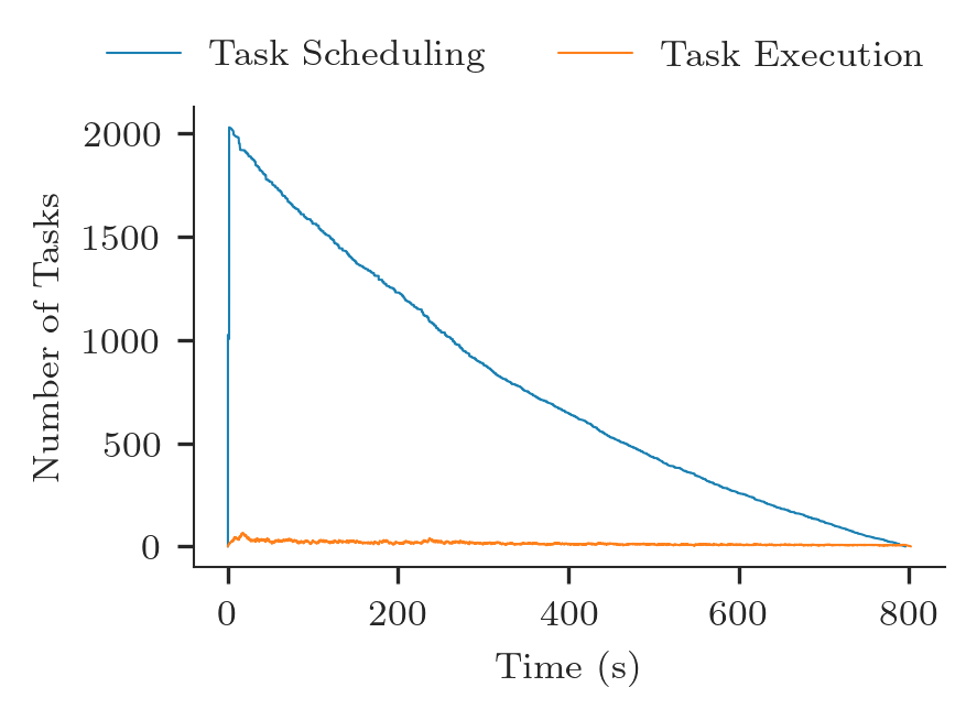
The plot above shows that tasks are between ‘AGENT_SCHEDULING’ and ‘schedule_ok’ at the beginning of the execution (dark blue). Few seconds later, tasks start to be between ‘rank_start’ and ‘rank_stop’, i.e., they are scheduled and start executing. Tasks appear to have a relatively heterogeneous duration, consistent with the task runtime distribution measured in duration analysis.

Task as scheduled as soon as new resources become available, across the whole duration of the workload execution. Consistently, the total number of tasks waiting to be scheduled progressively decreases, represented by the slope of the blue line. Consistently, the number of executed tasks remain relatively constant across all the workload duration, represented by the orange line.